Histogram and scatter plot
Exercise histogram-and-scatter-annex.pdf · PDF
Are most games on Steam cheap or expensive? You have 26,685 prices in games_clean. A bar per exact price would give you hundreds of bars: 0.99, 1.99, 2.49, 2.99... Nobody could read that.
Competitive games solved this problem long ago. In ranked mode, nobody plots one bar per player. The game cuts the rating scale into ranges, calls them Bronze, Silver, Gold, Platinum and Diamond, and counts how many players are in each. One look and you know where most people are, and how rare the top is.
That picture is the first chart of this lesson. The second one answers a different kind of question, also from ranked mode: do players with more hours have a higher rank? One number cannot answer that. You need two, on the same picture.
What you will learn
- Say what a histogram shows, and how it differs from a bar chart
- Choose a sensible number of bins, and see what outliers do to a histogram
- Read a distribution in words: where most values are, how long the tail is
- Build a scatter plot of two numeric columns and say what one dot stands for
- Describe a relationship (direction and strength) without claiming a cause
- Defuse the trap: why "the cloud rises" does not mean "one thing causes the other"
The histogram: the rank distribution
A histogram cuts one numeric column into equal ranges and draws one bar per range. The height of each bar is the number of rows that fall inside it.
Each range is a bin. The shape the bars draw together is the distribution of the column: where the values pile up and where they are rare.
In ranked mode, the numeric column is the rating, the bins are the ranks, and the height is the number of players. With game prices, the column is price, each bin is a price range, and the height is the number of games.
The word is older than video games: the English statistician Karl Pearson introduced the term histogram in 1891.
It looks like a bar chart. It is not
Both have bars, and that is where the similarity ends.
| Bar chart | Histogram | |
|---|---|---|
| X-axis | Categories that already exist (price_band) |
One numeric column cut into equal bins |
| Bar height | Any metric per category | Always a count: the rows inside the bin |
| You choose | The dimension and the metric | The column and the number of bins |
| Order of the bars | Yours to decide (sort by value) | Fixed: the number line, small to large |
| It answers | Which category is bigger? | What shape do the values have? Where are most of them? |
In Categorisation you built price_band by hand, with CASE WHEN. Those bands had unequal widths that you chose: Under 5, 5 to 15, 15 to 30. A histogram is different: it takes the minimum and the maximum of the data and cuts everything in between into bins of equal width.
That last detail is about to bite.
One giant bar: what outliers do
Ask for a histogram of price with 5 bins and you get the chart on the left.
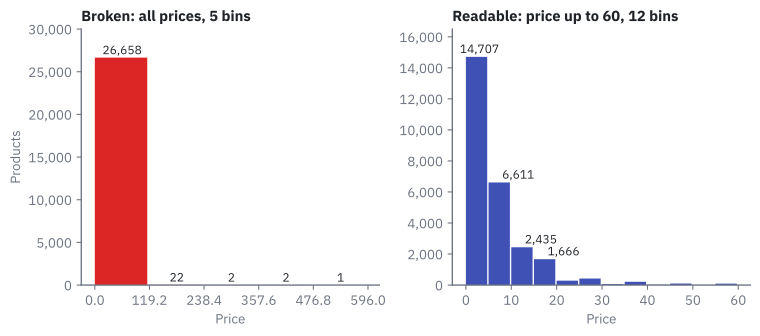
One enormous bar and almost nothing else: 26,658 products in the first bin, then 22, 2, 2 and 1. The chart is correct. It is also useless.
Why? Five equal bins between the cheapest and the most expensive product. So what is the most expensive?
SELECT game, price FROM games_clean ORDER BY price DESC LIMIT 6;
game |
price |
|---|---|
| ADR-Labelling Game | 595.99 |
| GameMaker Studio 2 UWP | 399.99 |
| VEGAS Pro 16 Edit Steam Edition | 399.00 |
| Marvelous Designer 8 for Steam | 320.00 |
| Facerig Studio for Individual Creators | 299.99 |
| Silhouette | 199.99 |
Look at the names. Most of these are not games: they are design and video software sold on Steam. A handful of rows stretch the axis to 595.99, so each of the 5 bins is 119.2 wide, and nearly every product in the table falls into the first one.
An outlier is a value that sits far away from almost all the others.
The fix has two parts: look only at the range where the games are, and use more bins. Filter to prices up to 60, ask for 12 bins, and you get the chart on the right. The filter leaves out only 83 of the 26,685 rows (0.3 %).
Careful: removing outliers from a picture is not deleting data
Those 83 rows are real products with real prices. You removed them from this chart because the question is about games, and you say so in the title: "price up to 60". An outlier is a value to investigate, not to delete by reflex. They are still in games_clean.
Reading a distribution in words
A histogram is finished when you can say it in one sentence. For the chart on the right:
Most games are cheap: 14,707 of 26,602 (55 %) cost less than 5, and that bar includes the 3,094 free games.
Three things to look for in any distribution:
| Look for | In the price histogram |
|---|---|
| Where is the peak? | The first bin, 0 to 5 |
| Is there a tail? The low part that stretches to one side | A long tail to the right: fewer and fewer games as the price rises |
| Anything odd? | A zigzag in the tail |
The zigzag has a boring explanation. Shops love prices ending in .99, and 24.99 and 29.99 land in different bins. Some bins contain a popular price and their neighbours do not.
This picture also explains something from Exploratory statistics. The mean price is 7.91 and the median is 4.99. Why so different? The long right tail: a few expensive products pull the mean up, while the median stays where most games are. The histogram is the picture of why they differ.
Careful: more bins is not always better
Too few bins hide the shape: with 5 bins you saw one bar. Too many turn the shape into noise, with hundreds of thin bars and gaps. Try two or three values and keep the one that tells the truth simply.
The scatter plot: one dot per player
Back to ranked mode. Do players with more hours have a higher rank? A histogram cannot answer: it looks at one number. Take every player, put their hours on the horizontal axis and their rank on the vertical axis, and draw a dot.
A scatter plot draws one dot per row, placed by two numeric columns: one sets the horizontal position, the other the vertical one. It shows the relationship between the two.
Here is a real one from the class table pokemon. Each of the 949 dots is one Pokémon, placed by its attack and its defense:
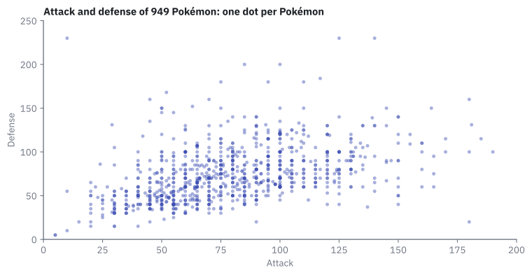
You do not read a scatter plot dot by dot. You read the shape of the cloud:
| Cloud shape | Reading | Careful |
|---|---|---|
| Rises to the right | Positive relationship: when one is high, the other tends to be high | It does not say which one causes the other |
| Falls to the right | Negative relationship: when one is high, the other tends to be low | Same warning |
| Round blob | No clear relationship | That is also an answer |
This cloud rises to the right, loosely: Pokémon with more attack tend to have more defense. Tend to. The cloud is wide, and some dots ignore the rule completely. The dot alone in the top-left corner is Shuckle: attack 10, defense 230.
How tight a cloud is has a number.
Correlation measures how closely two numbers move together, from -1 (a perfect falling line) through 0 (a blob) to 1 (a perfect rising line).
In PostgreSQL the function is CORR:
SELECT CORR(attack, defense) FROM pokemon;
It returns 0.44: a positive relationship of moderate strength. The scatter plot is the picture, and the correlation is its one-number summary. Always look at the picture too: in Data do not speak alone you saw four datasets with the same summary numbers and four completely different shapes.
Correlation is not causation
A scatter plot shows that two things go together. It never shows that one causes the other.
Causation means that changing one thing makes the other change. A chart alone cannot prove it.
Go back to ranked mode. Suppose players with more hours do have a higher rank. Does playing more make you better? Maybe. Or maybe good players enjoy the game more and so play more: the arrow points the other way. Or a third thing drives both.
The class data have a clean example. Among Steam games that have a review score, pricier games score a little higher. Does raising the price improve the reviews? Of course not. Big studios charge more and have bigger budgets. The budget sits behind both numbers.
flowchart TB
    B["<b>A third thing</b><br>a big studio<br>with a big budget"]
    B --> P["<b>Higher price</b>"]
    B --> M["<b>Better reviews</b>"]
    P -. "the chart shows these two together.<br>It does not show an arrow" .- M
Careful: the honest sentence
Say what the chart shows and nothing more. "Among reviewed games, pricier ones score a little higher on average" is honest. "Raise the price and the reviews improve" is a claim the chart cannot support.
Only the rows that have the value
There is one more trap in that price and review example, and it is about which rows are in the chart.
The review score is the column metascore. Only 2,849 of the 26,685 games have one: about 11 %. In Imputation you decided not to invent the missing scores, and you added the column has_metascore to tell the two groups apart.
So a chart of price against metascore describes those 2,849 games, not Steam. And they are not a random 11 %: critics review the games that get attention. Say it in the title.
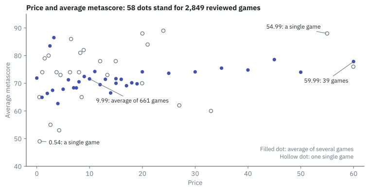
Here is what Superset draws when you ask for a scatter plot of price and the average metascore:
Careful: here each dot is one price, not one game
Superset's Scatter Plot groups by the X-axis. There are 58 dots, one per different price, and the height of a dot is the average metascore of all the reviewed games sold at that price. Compare with the Pokémon chart, where a dot was one Pokémon. Before reading any chart, ask: what does one mark stand for?
The cloud rises slightly. But look at which dots you can trust:
| Price | Average metascore | Games behind the dot |
|---|---|---|
| 0.00 | 71.9 | 159 |
| 4.99 | 67.8 | 202 |
| 9.99 | 71.6 | 661 |
| 19.99 | 74.1 | 504 |
| 29.99 | 74.1 | 165 |
| 39.99 | 74.8 | 75 |
| 59.99 | 77.8 | 39 |
| 0.54 (the lowest dot) | 49.0 | 1 |
| 54.99 | 88.0 | 1 |
The dot at 9.99 is the average of 661 games. The dot at 54.99 is one single game that happened to score 88. Superset draws both with the same size. In the figure above the single-game dots are hollow so that you can tell them apart: 26 of the 58 dots stand for only one game.
Game by game, the relationship is weak: CORR(price, metascore) over the 2,849 reviewed games is 0.16.
Try it: prices, and price against metascore
Both charts use the dataset games_clean (see Resources for the data).
Chart 4 — Price distribution. Where are most games, and how long is the tail?
| Step | Do this in Superset | You should see |
|---|---|---|
| 1 | New chart on games_clean, chart type Histogram. It is not in the first list (Featured): click All charts, or type histogram in the search box |
An empty chart editor |
| 2 | Column: price. Row limit: change 10000 to 50000. Leave Bins at 5. Create chart |
One enormous bar. Hover over it: 0 - 119.2 |
| 3 | Filters: price, operator Less or equal (<=), type 60 and pick it in the list, Save |
A chip price <= 60 under Filters |
| 4 | Bins: type 12 and press Enter. Update chart |
Twelve bars, the first one the tallest, a tail to the right |
| 5 | Customize, Y Axis Format: ,d |
The hover box says 14,707 instead of 14.7k |
| 6 | Save, name UT3 · Price distribution |
The chart is in the Charts list |
Do not skip the row limit in step 2. A histogram is computed from the rows it receives, and with the default it would read only 10,000 of your 26,685 games.
The twelve bars must match these counts:
| Bin starts at | Games | Bin starts at | Games | Bin starts at | Games |
|---|---|---|---|---|---|
| 0 | 14,707 | 20 | 282 | 40 | 18 |
| 5 | 6,611 | 25 | 419 | 45 | 99 |
| 10 | 2,435 | 30 | 60 | 50 | 6 |
| 15 | 1,666 | 35 | 209 | 55 | 90 |
Chart 5 — Price vs metascore. Do more expensive games get better reviews?
| Step | Do this in Superset | You should see |
|---|---|---|
| 1 | New chart on games_clean, chart type Scatter Plot |
An empty chart editor |
| 2 | X-axis: price. Metrics: Simple tab, column metascore, aggregate AVG |
The metric AVG(metascore) |
| 3 | Filters: has_metascore, operator Is true, Save. Create chart |
A cloud of 58 dots between 0 and 60 on the X-axis |
| 4 | Hover over the dot at 9.99, the dot at 59.99 and the lowest dot | 71.6, 77.8 and 49 |
| 5 | Save, name UT3 · Price vs metascore |
The chart is in the Charts list |
The dots are the 58 rows of this query:
SELECT price, ROUND(AVG(metascore)::numeric, 1) AS avg_metascore, COUNT(*) AS games
FROM games_clean WHERE has_metascore GROUP BY price ORDER BY price;
If something looks wrong
- The first bar ends near 40 instead of 119, or the bars add up to 10,000. Row limit is still at 10,000, so the chart read only part of the table. Set it to 50,000.
- Still one giant bar after the filter. The filter was not saved (the chip
price <= 60must appear under Filters), or Update chart was not pressed. - "Must specify a value for filters with comparison operators". The chip says
price <=with no number. Click it, type60, pick it in the list, Save. - A scatter with a single dot.
pricewent to Metrics instead of X-axis. - Dots spread evenly like a bar chart. Force categorical is ticked under the X-axis. Untick it.
Go further: the cumulative histogram
In the histogram, tick Cumulative and update the chart (do not save it). Each bar now adds all the bars before it. The second bar reaches 21,318: the first two bins together. So 80 % of these 26,602 games cost less than 10.
Key takeaways
- A histogram cuts one numeric column into equal bins and counts the rows in each. It shows a distribution: where the values pile up and how long the tail is.
- A histogram is not a bar chart: its X-axis is a number line, its height is always a count, and you choose the number of bins.
- Outliers stretch the axis and squash everything into one bar. Filter the chart to a sensible range, say so in the title, and do not delete the rows.
- A scatter plot places dots by two numeric columns and shows their relationship: rising, falling or none. Correlation puts a number on it.
- Correlation is not causation. Two things can move together because a third thing drives both.
- Always ask what one mark stands for and which rows are in the chart. Price against metascore describes the 11 % of games with a review, and each dot is a price, not a game.
Quick check
1. What does the height of a bar in a histogram always show?
- The average of the column inside that bin
- The number of rows whose value falls inside that bin
- The largest value inside that bin
- Any metric you choose, as in a bar chart
A histogram counts. Each bin is a range of one numeric column, and the bar height is how many rows fall in it. Choosing any metric per category is what a bar chart does.
2. How is a histogram of price different from the bar chart of price_band?
- There is no difference: both have bars
- The histogram uses colours and the bar chart does not
- The histogram cuts the number into equal-width bins computed from the data;
price_bandhas unequal bands chosen by hand - The bar chart can only show five bars
price_band was built with CASE WHEN and its widths were your choice. A histogram takes the minimum and the maximum of the data and makes equal-width bins, which is exactly why outliers can break it.
3. Your first histogram of price shows one giant bar and four almost empty ones. What is the cause?
- The column
priceis stored as text - Most games are free
- A few products priced up to 595.99 stretch the axis, so each of the 5 bins is 119.2 wide
- Superset can only draw one bar in a histogram
The bins are cut between the minimum and the maximum. A handful of outliers (expensive software, not games) push the maximum to 595.99, and 26,658 products land in the first bin.
4. You filter the histogram to price <= 60. What happened to the 83 products above 60?
- They were deleted from
games_clean - They were moved into the last bin
- They are still in the table; they were left out of this chart, and the title should say so
- Their price was changed to 60
A chart filter changes the picture, not the data. The rows are real and stay in the table. An outlier is a value to investigate, not to delete by reflex.
5. In the Pokémon scatter plot, the cloud rises loosely to the right and CORR(attack, defense) is 0.44. What can you say?
- Raising a Pokémon's attack causes its defense to rise
- Pokémon with more attack tend to have more defense, with many exceptions
- Every Pokémon with high attack has high defense
- Attack and defense are unrelated
A rising cloud is a positive relationship, and 0.44 says it is of moderate strength: a tendency, not a rule. Shuckle has attack 10 and defense 230. And a relationship never proves a cause.
6. In Superset's scatter plot of price against average metascore, what is one dot?
- One game
- One publisher
- One price: the average metascore of all reviewed games sold at that price
- One review written by a critic
Superset's Scatter Plot groups by the X-axis, so there are 58 dots for 2,849 games. The dot at 9.99 averages 661 games; the dot at 54.99 is a single game. Always ask what one mark stands for.
7. Why can you not say \"on Steam, expensive games get better reviews\" from that chart?
- Because the correlation is negative
- Because the chart only includes the roughly 11 % of games that have a metascore, and those are not a random sample
- Because scatter plots cannot use prices
- Because the chart has too few bins
Only 2,849 of 26,685 games have a metascore, and critics review the games that get attention. The chart describes reviewed games. A second problem: even there, a relationship is not a cause.
8. A friend shows you a histogram of the salaries in a company: one huge bar on the left and nothing else visible. Then they plot salary against years in the company and say \"staying longer makes you earn more\". Pick the two correct replies.
- A few very high salaries stretch the axis: filter to a sensible maximum, say so, and use more bins
- The scatter shows that salary and years go together, not that one causes the other
- The histogram is broken because salaries are categories
- The scatter proves the cause, because the cloud rises
The giant bar is the outlier effect you saw with prices, and the fix is the same. The second claim confuses correlation with causation: the two move together, and something else (the kind of job, for example) could drive both.
You can now show how one number spreads and how two numbers relate. Two famous charts are still missing, and one of them is very easy to get wrong: Pie, heatmap and others.