Exploratory statistics
Exercise exploratory-statistics-annex.pdf · PDF
Without running anything: how much does a typical game on Steam cost? Say a number. Write it down, even.
You have spent weeks cleaning games_clean. You know its columns by heart. And still you have to guess, because nobody has asked the table a single question yet. Today you ask. The answer is going to be two numbers that disagree with each other, and understanding why they disagree is the most useful piece of statistics you will ever learn.
What you will learn
- Compute the mean and the median of a column in SQL, and say which one a single extreme value moves
- Describe the spread of a column: minimum, maximum, quartiles and standard deviation
- Build a frequency table with
width_bucketand read the shape of a distribution from it - Tell a skewed column from a symmetric one just by comparing mean and median
- Choose the number that honestly answers "what is typical?"
- The trap: why "the average game costs 7.91" describes a game that barely exists
Today you produce the numbers; the next lesson turns them into the report.
The queue: two kinds of middle
Exploratory statistics means describing a column with a handful of numbers before you draw or conclude anything: where its middle is, how spread out it is, and what shape it has.
Five friends compare what they earn in a month. Four have ordinary jobs. The fifth is a streamer who had a very good month.
1 200 1 300 1 400 1 500 30 000
What does a typical friend earn? There are two honest ways to answer.
The mean (the everyday "average") is what each one would get if everything were added up and split equally.
Add the five: 35,400. Split by five: 7,080.
The median is the value of the one standing in the middle when everybody queues up from smallest to largest.
Put them in a queue by income. The third of five is in the middle: 1,400.
| How | Here | What the streamer does to it | |
|---|---|---|---|
| Mean | Add everything, split it equally | 7,080 | Drags it up. Nobody in the group earns anything near 7,080 |
| Median | Queue by size, take the one in the middle | 1,400 | Nothing. The streamer is just "the last one in the queue", whatever they earn |
Give the streamer 300,000 instead of 30,000. The mean jumps to 61,080. The median is still 1,400.
We keep the queue for the whole page. Put the data in a queue, smallest first. Half are in front of the median, half behind. Everything you compute today is a question about that queue:
| Question | In the queue | SQL |
|---|---|---|
| Centre | Where is the middle? | AVG, PERCENTILE_CONT(0.5) |
| Spread | How far apart are the first and the last? And the middle half? | MIN, MAX, STDDEV, percentiles 0.25 and 0.75 |
| Shape | Where does the queue bunch up? | width_bucket + COUNT(*) |
Centre: the same on 26,685 games
Now the real queue. Before you run it, bet: will the mean price be above or below the median?
SELECT ROUND(AVG(price), 2)                               AS mean,
       PERCENTILE_CONT(0.5) WITHIN GROUP (ORDER BY price) AS median
FROM games_clean;
| mean | median |
|---|---|
| 7.91 | 4.99 |
The mean is AVG, an old friend from SQL Lab: groups. The median needs a longer line. Read it piece by piece:
| Piece | In the queue |
|---|---|
WITHIN GROUP (ORDER BY price) |
"Make the queue by price" |
PERCENTILE_CONT(0.5) |
"Walk to 50% of the queue and read the value there" |
A percentile is a position in the queue, given as a fraction: 0.5 is the middle, 0.25 is a quarter of the way in.
PostgreSQL has no MEDIAN() function. The median is percentile 0.5.
So which is it: does a game cost 7.91 dollars or 4.99? Both numbers are correct. They answer different questions. To see which question, you need the rest of the queue.
Spread: how far apart
A centre alone hides too much. "The middle game costs 4.99" is true whether every game costs 4.99 or whether prices run from zero to hundreds. Start with the two ends of the queue:
SELECT COUNT(*) AS n, MIN(price) AS lowest, MAX(price) AS highest,
       ROUND(AVG(price), 2) AS mean,
       PERCENTILE_CONT(0.5) WITHIN GROUP (ORDER BY price) AS median
FROM games_clean;
| n | lowest | highest | mean | median |
|---|---|---|---|---|
| 26,685 | 0.00 | 595.99 | 7.91 | 4.99 |
A game at 595.99? Never report a maximum without looking at who it is:
SELECT game, price FROM games_clean ORDER BY price DESC LIMIT 3;
| game | price |
|---|---|
| ADR-Labelling Game | 595.99 |
| GameMaker Studio 2 UWP | 399.99 |
| VEGAS Pro 16 Edit Steam Edition | 399.00 |
The second is a tool for making games and the third is a video editor. They are software sold on Steam, not games. These are the streamers of our queue.
The ends of the queue are set by one row each. A sturdier way to describe spread is to cut the queue in four equal parts.
The quartiles are the three cuts that split the queue into four parts with the same number of rows: Q1 at 25%, the median at 50%, Q3 at 75%.
The standard deviation is, roughly, the typical distance between a value and the mean. (The exact formula squares the distances first; you do not need it today, and
STDDEVdoes it for you.)
SELECT ROUND(STDDEV(price), 2) AS std_dev,
       PERCENTILE_CONT(0.25) WITHIN GROUP (ORDER BY price) AS q1,
       PERCENTILE_CONT(0.75) WITHIN GROUP (ORDER BY price) AS q3
FROM games_clean;
| std_dev | q1 | q3 |
|---|---|---|
| 11.79 | 1.99 | 9.99 |
Between Q1 and Q3 stands the middle half of the queue. So you can write a sentence that is short, exact and true: half of all games cost between 1.99 and 9.99 dollars.
Careful: the standard deviation is not a price range
It is tempting to read "mean 7.91, standard deviation 11.79" as "prices go from 7.91 − 11.79 to 7.91 + 11.79". The lower end would be negative, and no game costs less than nothing. On a column like this one, the standard deviation is inflated by the few huge values at the end of the queue. The quartiles describe the spread better.
Shape: where the queue bunches up
Centre and spread are still only numbers. To see the queue you need its shape.
A distribution is how the values of a column are shared out: which values are common and which are rare.
The simplest way to see it is a frequency table: cut the range into boxes of equal width and count how many rows fall in each box.
width_bucket(value, from, to, n) tells you which of n equal boxes between from and to a value falls in. Below: six boxes of 10 dollars from 0 to 60. Anything above 60 goes to an extra box, number 7. The last column draws a bar: one # for every 500 games.
SELECT width_bucket(price, 0, 60, 6) AS bucket,
       MIN(price) AS lowest, MAX(price) AS highest, COUNT(*) AS games,
       REPEAT('#', (COUNT(*) / 500)::int) AS bar
FROM games_clean GROUP BY bucket ORDER BY bucket;
 bucket | lowest | highest | games | bar
--------+--------+---------+-------+--------------------------------------------
      1 |   0.00 |    9.99 | 21318 | ##########################################
      2 |  10.00 |   19.99 |  4101 | ########
      3 |  20.00 |   29.99 |   701 | #
      4 |  30.00 |   39.99 |   269 |
      5 |  40.00 |   49.99 |   117 |
      6 |  54.99 |   59.99 |    96 |
      7 |  64.99 |  595.99 |    83 |
There is the queue. Almost everybody is crammed into the first box: 21,318 games out of 26,685 cost less than 10 dollars. Then a long, thin line of stragglers stretches to the right, all the way to 595.99.
Why does box 6 start at 54.99 and not at 50?
The columns lowest and highest show the cheapest and the dearest game found in each box, not the edges of the box. Box 6 covers 50 to 60, but no game in this table costs between 50.00 and 54.98.
Do the same for a second column, metascore, the review score from 0 to 100. Two changes: only the games that have a score (WHERE has_metascore), and a cast to numeric, because ROUND with decimals does not accept the type of that column directly.
SELECT COUNT(*) AS n, MIN(metascore) AS lowest, MAX(metascore) AS highest,
       ROUND(AVG(metascore)::numeric, 1) AS mean,
       PERCENTILE_CONT(0.5) WITHIN GROUP (ORDER BY metascore) AS median,
       ROUND(STDDEV(metascore)::numeric, 1) AS std_dev,
       PERCENTILE_CONT(0.25) WITHIN GROUP (ORDER BY metascore) AS q1,
       PERCENTILE_CONT(0.75) WITHIN GROUP (ORDER BY metascore) AS q3
FROM games_clean WHERE has_metascore;
| n | lowest | highest | mean | median | std_dev | q1 | q3 |
|---|---|---|---|---|---|---|---|
| 2,849 | 20 | 98 | 71.9 | 73 | 11.0 | 66 | 80 |
SELECT width_bucket(metascore, 20, 100, 8) AS bucket,
       MIN(metascore) AS lowest, MAX(metascore) AS highest, COUNT(*) AS games,
       REPEAT('#', (COUNT(*) / 25)::int) AS bar
FROM games_clean WHERE has_metascore GROUP BY bucket ORDER BY bucket;
 bucket | lowest | highest | games | bar
--------+--------+---------+-------+--------------------------------------------
      1 |     20 |      29 |     8 |
      2 |     30 |      39 |    21 |
      3 |     40 |      49 |    85 | ###
      4 |     50 |      59 |   261 | ##########
      5 |     60 |      69 |   666 | ##########################
      6 |     70 |      79 |  1055 | ##########################################
      7 |     80 |      89 |   677 | ###########################
      8 |     90 |      98 |    76 | ###
A completely different queue. This one is a hill: few games at the bottom, few at the top, and a crowd in the middle, between 70 and 79.
Two shapes: the tail and the hill
Here are both frequency tables as a picture, with the mean and the median marked.
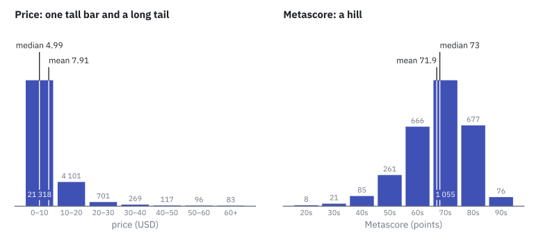
A distribution is skewed when most values pile up on one side and a long tail of rare values stretches out on the other. It is symmetric when both sides of the centre look roughly alike.
price |
metascore |
|
|---|---|---|
| Shape | One tall bar and a long tail to the right: skewed | A hill: roughly symmetric |
| Mean | 7.91 | 71.9 |
| Median | 4.99 | 73 |
| Mean vs median | Far apart: the mean is 58% higher | Close together: about one point apart |
| Who pulls the mean | 83 products at 60 dollars or more, up to 595.99 | Nobody in particular |
Now you can tell the shape without drawing anything. Compare the two centres. Far apart means there is a tail, and the mean has been dragged towards it. Close together means a hill.
Careful: the average is not always the typical value
"Most games cost about 7.91" sounds reasonable and is false. Only 10,218 of the 26,685 games cost more than the mean; 62% cost less. It is the streamer effect: a few very expensive products pull the mean away from where the queue actually stands.
When mean and median disagree, the median describes the typical case and the mean describes the total (multiply it by the number of games and you get the sum of all prices). Neither is wrong. They answer different questions.
Which number do we print?
Go back to the number you wrote down at the start. Were you close? Close to which one?
In the next lesson you write a report, and one line of it will say what a game costs. If you print 7.91, you describe a game that barely exists. Here is the same fact, written three ways:
| Sentence | Verdict |
|---|---|
| "The average price is 7.91." | True, and misleading: no unit, and no warning that most games cost less |
| "Games cost around 5 dollars." | Closer, but vague: which number is that, and how sure are you? |
| "The typical game costs 4.99 USD (median). Half of all games cost between 1.99 and 9.99 USD. The mean is higher, 7.91 USD, because a few products cost up to 595.99 USD." | The centre, the spread and the shape, in three short sentences |
A number without its shape is half a truth. Print the median, the quartiles, and say in words that there is a tail.
Try it
Use games_clean in SQL Lab (database Dades classe, schema public). Build your own stat card: a small table with eight numbers per column.
| n | lowest | highest | mean | median | std_dev | Q1 | Q3 | |
|---|---|---|---|---|---|---|---|---|
price |
||||||||
metascore |
Step 1 — Run the queries of this page and fill in both rows. Your numbers must match the ones above.
Step 2 — Count how many games cost more than the mean, with WHERE price > 7.91. You should get 10,218.
Step 3 — On paper, sketch the seven bars of price and the eight bars of metascore. Mark where the mean and the median fall on each sketch.
Step 4 — Do Hit games cost more? Add a group to the first query:
SELECT owners_tier, ROUND(AVG(price), 2) AS mean,
       PERCENTILE_CONT(0.5) WITHIN GROUP (ORDER BY price) AS median
FROM games_clean GROUP BY owners_tier;
| owners_tier | mean | median |
|---|---|---|
| Hit | 13.99 | 9.99 |
| Mid | 8.60 | 4.99 |
| Niche | 7.38 | 4.99 |
Step 5 — Finish the two sentences: "A typical game costs __ because..." and "A typical reviewed game scores __ because...". Keep the card: it is the raw material of your report.
If SQL Lab complains
function round(double precision, integer) does not exist means you are rounding the metascore column as it is. Cast it first: ROUND(AVG(metascore)::numeric, 1). And if a row with an empty bucket appears, the WHERE has_metascore is missing: games without a score fall in no box.
Key takeaways
- Exploratory statistics describes a column with a few numbers: centre, spread and shape.
- The mean adds everything and splits it equally; the median is the middle of the queue. One extreme value moves the mean and leaves the median where it was.
- PostgreSQL has no
MEDIAN(): usePERCENTILE_CONT(0.5) WITHIN GROUP (ORDER BY column). The quartiles Q1 and Q3 are percentiles 0.25 and 0.75. - A frequency table with
width_bucketandCOUNT(*)shows the distribution: where the values bunch up. priceis skewed (mean 7.91, median 4.99, a tail up to 595.99).metascoreis roughly symmetric (mean 71.9, median 73).- Mean and median far apart means a tail. For a skewed column, report the median and the quartiles, and say that there is a tail.
Quick check
1. Five friends earn 1,200, 1,300, 1,400, 1,500 and 30,000. The last one's income rises to 300,000. What happens?
- Both the mean and the median rise
- The mean rises a lot; the median stays at 1,400
- The median rises a lot; the mean stays at 7,080
- Neither changes, because it is only one person
The mean adds everything up, so one huge value drags it: from 7,080 to 61,080. The median only cares about who stands in the middle of the queue. The streamer is still "the last one", whatever they earn.
2. Which SQL gives the median price in PostgreSQL?
-
AVG(price) -
(MIN(price) + MAX(price)) / 2 -
PERCENTILE_CONT(0.5) WITHIN GROUP (ORDER BY price) -
STDDEV(price)
The median is percentile 0.5: make the queue by price, walk to 50% of it and read the value. Halfway between the lowest and the highest would be about 298, a price almost no game has. The real median is 4.99.
3. The mean price is 7.91 and the median is 4.99. What does the gap tell you?
- That one of the two queries has a mistake
- That half of the games cost exactly 7.91
- That the distribution is skewed: a tail of expensive products pulls the mean up
- That prices are spread evenly between 4.99 and 7.91
When mean and median are far apart, there is a tail. Here 83 products cost 60 dollars or more, up to 595.99, and they drag the mean. In metascore, a hill, the two centres are about one point apart.
4. Q1 of price is 1.99 and Q3 is 9.99. Which sentence is correct?
- Half of all games cost between 1.99 and 9.99
- A quarter of all games cost between 1.99 and 9.99
- No game costs less than 1.99 or more than 9.99
- The mean must be exactly halfway, at 5.99
The quartiles cut the queue in four equal parts. Between Q1 (25%) and Q3 (75%) stands the middle half of the rows. A quarter of the games are cheaper than Q1 and another quarter are dearer than Q3.
5. A classmate writes: most games cost about 7.91, the average. What is wrong with this sentence?
- Nothing: the average is always the typical value
- The average is really 4.99
- Only 10,218 of 26,685 games cost more than 7.91; 62% cost less
- An average cannot be computed on prices
The arithmetic is right, the reading is wrong. On a skewed column the mean sits above most of the rows. The median, 4.99, describes the typical game; the mean describes the total.
6. What does width_bucket(price, 0, 60, 6) do?
- It rounds every price to the nearest 6 dollars
- It keeps only the six cheapest games
- It says which of six equal boxes between 0 and 60 each price falls in
- It splits the table into six tables
Six boxes of 10 dollars each. Together with GROUP BY and COUNT(*) it builds a frequency table, which shows the shape of the distribution. Prices of 60 or more land in an extra box, number 7.
7. A town has 99 flats rented at 700 to 900 euros a month (about 800 on average) and one mansion at 40,000. The newspaper prints: average rent, about 1,190 euros. Pick the two true statements.
- The figure is arithmetically right, but 99 of 100 tenants pay less than it
- The median, about 800 euros, describes the typical rent better
- The figure is false: the newspaper made a calculation error
- The mansion should be counted twice so that the average is fair
It is the streamer again. (99 × 800 + 40,000) ÷ 100 ≈ 1,190, so the mean is correct and describes nobody. Print the median, PERCENTILE_CONT(0.5) WITHIN GROUP (ORDER BY rent), and mention the range of the middle half.
You now have a card full of honest numbers. Numbers alone are not a report, though. Next: The descriptive report, where you turn the stat card into a page someone else can trust.